Package: xcms
Authors: Johannes Rainer, Mar Garcia-Aloy
Modified: 2021-03-03 10:06:56
Compiled: Wed Mar 3 11:01:34 2021
Introduction
In a typical LC-MS-based metabolomics experiment compounds eluting from the chromatography are first ionized before being measured by mass spectrometry (MS). During the ionization different (multiple) ions can be generated from the same compound which all will be measured by MS. In general, the resulting data is then pre-processed to identify chromatographic peaks in the data and to group these across samples in the correspondence analysis. The result are distinct LC-MS features, characterized by their specific m/z and retention time range. Different ions generated during ionization will be detected as different features. To reduce data set complexity (and to aid in subsequent annotation steps) it is advisable to group features which are supposedly representing signal from the same original ion. This document describes functionality to aid in this feature grouping step which are provided by this package.
LC-MS feature grouping
We demonstrate the feature grouping functionality on the simple toy data set used also in the xcms package and provided through the faahKO package. This data set consists of samples from 4 mice with knock-out of the fatty acid amide hydrolase (FAAH) and 4 wild type mice. Pre-processing of this data set is described in detail in the xcms vignette of the xcms package. Below we load all required packages and the result from this pre-processing updating also the location of the respective raw data files on the current machine.
library(xcms)
library(faahKO)
library(MsFeatures)
library(CompMetaboTools)

data("xdata")
## Update the path to the files for the local system
dirname(xdata) <- paste0(system.file("cdf/", package = "faahKO"),
                         rep(c("/KO/", "/WT/"), each = 4))
Before performing the feature grouping we inspect the result object. With featureDefinitions we can extract the results from the correspondence analysis.
featureDefinitions(xdata)## DataFrame with 225 rows and 11 columns
## mzmed mzmin mzmax rtmed rtmin rtmax npeaks
## <numeric> <numeric> <numeric> <numeric> <numeric> <numeric> <numeric>
## FT001 200.1 200.1 200.1 2901.63 2880.73 2922.53 2
## FT002 205.0 205.0 205.0 2789.39 2782.30 2795.36 8
## FT003 206.0 206.0 206.0 2788.73 2780.73 2792.86 7
## FT004 207.1 207.1 207.1 2718.12 2713.21 2726.70 7
## FT005 219.1 219.1 219.1 2518.82 2517.40 2520.81 3
## ... ... ... ... ... ... ... ...
## FT221 591.30 591.3 591.3 3005.03 2992.87 3006.05 5
## FT222 592.15 592.1 592.3 3022.11 2981.91 3107.59 6
## FT223 594.20 594.2 594.2 3418.16 3359.10 3427.90 3
## FT224 595.25 595.2 595.3 3010.15 2992.87 3013.77 6
## FT225 596.20 596.2 596.2 2997.91 2992.87 3002.95 2
## KO WT peakidx ms_level
## <numeric> <numeric> <list> <integer>
## FT001 2 0 287, 679,1577,... 1
## FT002 4 4 47,272,542,... 1
## FT003 3 4 32,259,663,... 1
## FT004 4 3 19,249,525,... 1
## FT005 1 2 639, 788,1376,... 1
## ... ... ... ... ...
## FT221 2 3 349,684,880,... 1
## FT222 1 3 86,861,862,... 1
## FT223 1 2 604, 985,1543,... 1
## FT224 2 3 67,353,876,... 1
## FT225 0 2 866,1447,1643,... 1Each row in this data frame represents the definition of one feature, with its average and range of m/z and retention time. Column "peakidx" provides the index of each chromatographic peak which is assigned to the feature in the chromPeaks matrix of the result object. The featureValues function allows to extract feature values, i.e. a matrix with feature abundances, one row per feature and columns representing the samples of the present data set.
Below we extract the feature values with and without filled-in peak data. Without the gap-filled data only abundances from detected chromatographic peaks are reported, with gap-filled data, for samples in which no chromatographic peak was identified (e.g. because peak detection failed for that ion in that particular sample) data was filled-in in samples in which no peak was detected integrating all signal from the MS region defined by the m/z - retention time range of the detected chromatographic peak in the other samples.
head(featureValues(xdata, filled = FALSE))## ko15.CDF ko16.CDF ko21.CDF ko22.CDF wt15.CDF wt16.CDF wt21.CDF
## FT001 NA 506848.9 NA 169955.6 NA NA NA
## FT002 1924712.0 1757151.0 1383416.7 1180288.2 2129885.1 1634342.0 1623589.2
## FT003 213659.3 289500.7 NA 178285.7 253825.6 241844.4 240606.0
## FT004 349011.5 451863.7 343897.8 208002.8 364609.8 360908.9 NA
## FT005 NA NA NA 107348.5 223951.8 NA NA
## FT006 286221.4 NA 164009.0 149097.6 255697.7 311296.8 366441.5
## wt22.CDF
## FT001 NA
## FT002 1354004.93
## FT003 185399.47
## FT004 221937.53
## FT005 84772.92
## FT006 271128.02
head(featureValues(xdata, filled = TRUE))## ko15.CDF ko16.CDF ko21.CDF ko22.CDF wt15.CDF wt16.CDF wt21.CDF
## FT001 159738.1 506848.88 113441.08 169955.6 216096.6 145509.7 230477.9
## FT002 1924712.0 1757150.96 1383416.72 1180288.2 2129885.1 1634342.0 1623589.2
## FT003 213659.3 289500.67 162897.19 178285.7 253825.6 241844.4 240606.0
## FT004 349011.5 451863.66 343897.76 208002.8 364609.8 360908.9 223322.5
## FT005 135978.5 25524.79 71530.84 107348.5 223951.8 134398.9 190203.8
## FT006 286221.4 289908.23 164008.97 149097.6 255697.7 311296.8 366441.5
## wt22.CDF
## FT001 140551.30
## FT002 1354004.93
## FT003 185399.47
## FT004 221937.53
## FT005 84772.92
## FT006 271128.02In total 225 features have been defined in the present data set, many of which most likely represent signal from different ions of the same compound. The aim of the grouping functions of this package are now to define which features most likely come from the same original compound. These feature grouping functions base on the following assumptions/properties of LC-MS data:
- Features (ions) of the same compound should have similar retention time.
- The peak shape of extracted ion chromatograms (EIC) of features of the same compound should be similar as it should follow the elution pattern of the original compound from the chromatogram.
- The abundance of features (ions) of the same compound should have a similar pattern across samples, i.e. if a compound is highly concentrated in one sample and low in another, all ions from it should follow the same pattern.
The main method to perform the feature grouping is called groupFeatures which takes an XCMSnExp object (result object from the xcms pre-processing) as input as well as a parameter object to chose the grouping algorithm and specify its settings. At present the following approaches are supported:
-
SimilarRtimeParam: perform an initial grouping based on similar retention time. -
EicCorrelationParam: perform a feature grouping based on correlation of EICs. -
AbundanceSimilarityParam: perform a feature grouping based on correlation of feature abundances (values) across samples.
Calling groupFeatures on an xcms result object will perform a feature grouping assigning each feature in the data set to a feature group. These feature groups are stored as an additional columns called "feature_group" in the featureDefinition data frame of the result object. Any subsequent groupFeature call will sub-group (refine) the identified feature groups further. It is thus possible to use a single grouping approach, or to combine multiple of them to generate the desired feature grouping. While the individual feature grouping algorithms can be called in any order, it is advised to use the EicCorrelationParam as last refinement step, because it is the computationally most expensive one, especially if applied to a result object without any pre-defined feature groups or if the feature groups are very large. In the subsequent sections we will apply the various feature grouping approaches subsequently.
Note also that we perform here a grouping of all defined features, but it would also be possible to just group a subset of interesting features (e.g. features found significant by a statistical analysis of the data set). How this can be achieved is described in the last section of this vignette.
Grouping of features by similar retention time
The most intuitive and simple way to group features is based on their retention time. Before we perform this initial grouping we evaluate retention times and m/z of all features in the present data set.
plot(featureDefinitions(xdata)$rtmed, featureDefinitions(xdata)$mzmed,
     xlab = "retention time", ylab = "m/z", main = "features",
     col = "#00000080")
grid()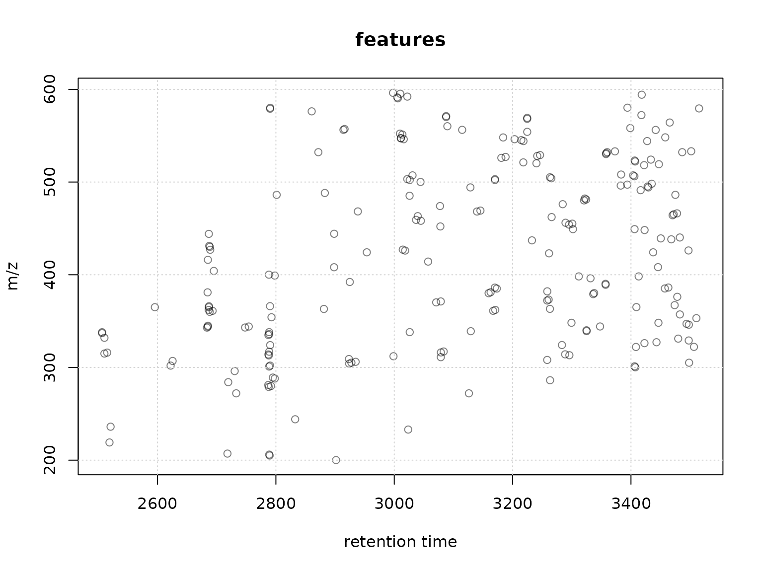
Plot of retention times and m/z for all features in the data set.
Especially in the earlier retention time range we can see features with about the same retention time. We below group features within a retention time window of 10 seconds.
xdata <- groupFeatures(xdata, param = SimilarRtimeParam(10))The results from the feature grouping can be accessed with the featureGroups function. Below we determine the size of each of these feature groups (i.e. how many features are grouped together).
table(featureGroups(xdata))##
## FG.001 FG.002 FG.003 FG.004 FG.005 FG.006 FG.007 FG.008 FG.009 FG.010 FG.011
## 3 3 3 3 2 4 5 6 4 2 5
## FG.012 FG.013 FG.014 FG.015 FG.016 FG.017 FG.018 FG.019 FG.020 FG.021 FG.022
## 3 4 3 5 3 3 5 3 3 3 3
## FG.023 FG.024 FG.025 FG.026 FG.027 FG.028 FG.029 FG.030 FG.031 FG.032 FG.033
## 3 3 6 3 3 3 3 2 3 3 4
## FG.034 FG.035 FG.036 FG.037 FG.038 FG.039 FG.040 FG.041 FG.042 FG.043 FG.044
## 3 2 2 3 2 2 4 2 2 2 3
## FG.045 FG.046 FG.047 FG.048 FG.049 FG.050 FG.051 FG.052 FG.053 FG.054 FG.055
## 4 2 3 3 3 2 2 3 4 2 3
## FG.056 FG.057 FG.058 FG.059 FG.060 FG.061 FG.062 FG.063 FG.064 FG.065 FG.066
## 2 2 2 3 2 3 2 2 2 3 2
## FG.067 FG.068 FG.069 FG.070 FG.071 FG.072 FG.073 FG.074 FG.075 FG.076 FG.077
## 2 3 2 2 2 3 2 2 1 1 1
## FG.078 FG.079 FG.080 FG.081 FG.082 FG.083 FG.084
## 1 1 1 1 1 1 1Below we plot the results from this feature grouping. Features being grouped together are connected with a line.
plotFeatureGroups(xdata)
grid()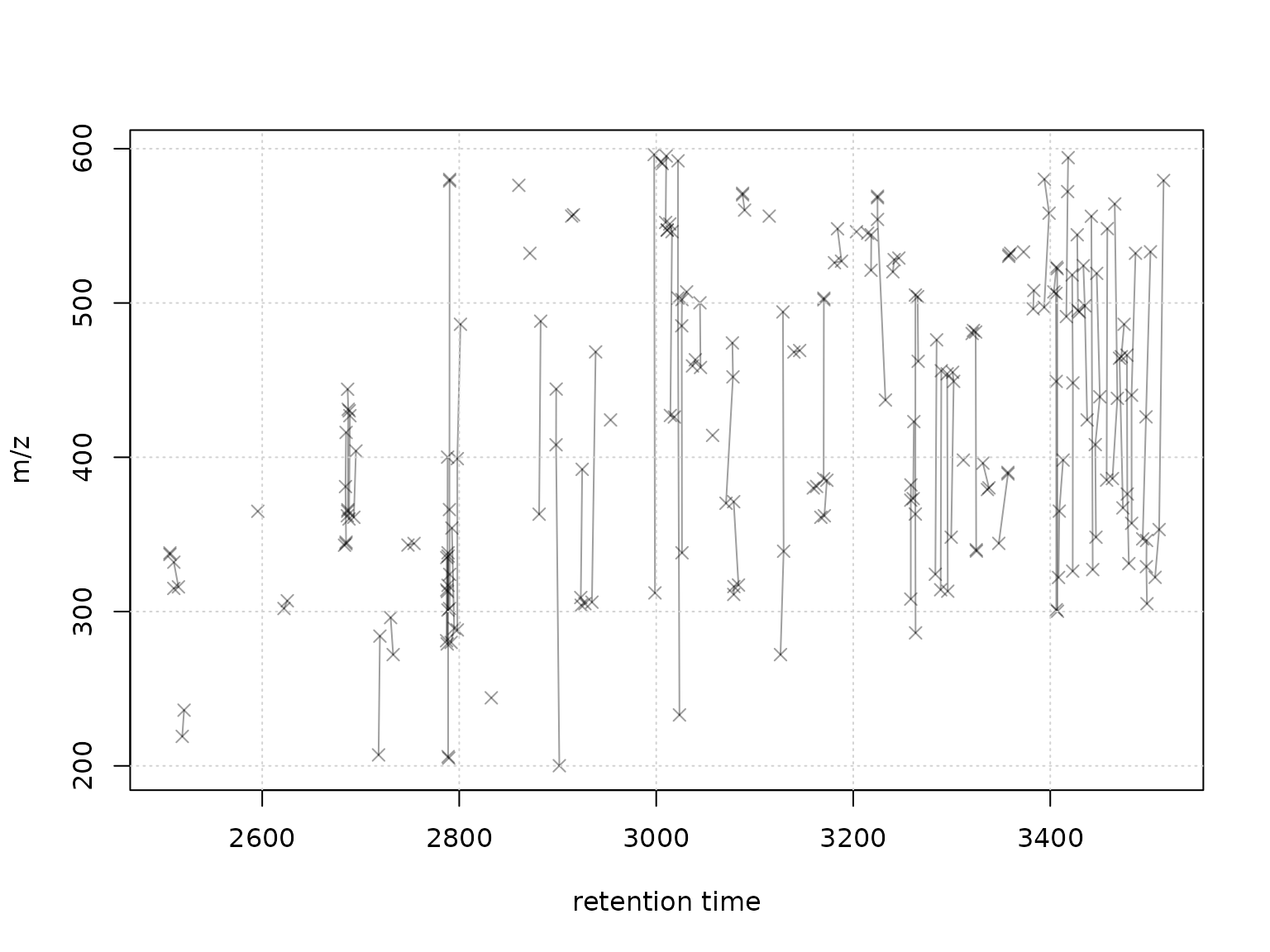
Feature groups defined with a rt window of 10 seconds
Let’s assume we are not totally happy with this feature grouping, also knowing that there were quite some shifts in retention times between runs. We thus re-perform the feature grouping based on similar retention time with a larger rt window. Before we have however to remove the previous results to avoid that these previous feature groups are simply refined with the following groupFeatures call.
## Remove previous feature grouping results to repeat the rtime-based
## feature grouping with different setting
featureDefinitions(xdata)$feature_group <- NULL

## Repeat the grouping
xdata <- groupFeatures(xdata, SimilarRtimeParam(20))
table(featureGroups(xdata))
##
## FG.001 FG.002 FG.003 FG.004 FG.005 FG.006 FG.007 FG.008 FG.009 FG.010 FG.011
## 3 3 3 3 2 4 5 6 4 2 5
## FG.012 FG.013 FG.014 FG.015 FG.016 FG.017 FG.018 FG.019 FG.020 FG.021 FG.022
## 3 4 3 5 3 3 5 3 3 3 3
## FG.023 FG.024 FG.025 FG.026 FG.027 FG.028 FG.029 FG.030 FG.031 FG.032 FG.033
## 3 3 6 3 3 3 4 2 3 3 4
## FG.034 FG.035 FG.036 FG.037 FG.038 FG.039 FG.040 FG.041 FG.042 FG.043 FG.044
## 3 2 3 3 2 2 4 3 2 2 4
## FG.045 FG.046 FG.047 FG.048 FG.049 FG.050 FG.051 FG.052 FG.053 FG.054 FG.055
## 4 2 3 3 3 2 2 3 4 2 3
## FG.056 FG.057 FG.058 FG.059 FG.060 FG.061 FG.062 FG.063 FG.064 FG.065 FG.066
## 3 2 2 3 3 3 2 2 2 3 2
## FG.067 FG.068 FG.069 FG.070 FG.071 FG.072 FG.073 FG.074 FG.075 FG.076 FG.077
## 2 3 2 2 3 3 2 2 1 1 1
plotFeatureGroups(xdata)
grid()
Feature groups defined with a rt window of 20 seconds
Note that this grouping approach uses the groupClosest function which can group arbitrary numeric values together based on their similarity. Thus, the same grouping could also be achieved on a simple single numeric vector of retention times:
groupClosest(featureDefinitions(xdata)$rtmed, 20)## [1] 21 1 1 57 62 19 62 75 44 66 23 48 3 57 16 14 48 66 30 4 15 11 69 33 33
## [26] 25 71 69 2 33 13 50 23 38 3 43 12 12 13 4 13 47 72 11 54 24 58 25 32 12
## [51] 3 1 5 5 6 4 28 44 28 7 74 7 22 74 7 25 25 45 52 72 48 20 27 8 64
## [76] 18 8 16 60 18 76 47 18 11 53 37 13 2 42 32 61 70 61 7 70 2 8 46 65 8
## [101] 22 22 33 61 56 47 14 23 64 45 21 36 7 42 71 59 40 25 27 40 27 18 9 65 45
## [126] 20 18 21 24 52 15 37 38 52 43 36 67 35 67 53 53 32 73 71 73 37 54 56 28 56
## [151] 6 53 14 60 34 49 44 49 41 26 59 36 8 6 8 19 35 16 15 15 6 41 24 45 55
## [176] 29 30 15 59 68 68 55 55 31 31 31 20 60 25 41 29 49 29 29 40 10 10 68 46 40
## [201] 39 9 58 63 44 63 26 17 65 9 9 17 17 34 77 11 72 11 26 51 51 19 34 39 50Grouping by similar retention time grouped the in total 225 features into 77 feature groups.
Grouping of features by abundance correlation across samples
Assuming we are OK with the crude initial feature grouping from the previous section, we can next refine the feature groups considering also the feature abundances across samples. We can use the groupFeatures method with an AbundanceSimilarityParam object. This approach performs a pairwise correlation between the feature values (abundances; across samples) between all features of a predefined feature group (such as defined in the previous section). Features that have a correlation >= threshold are grouped together. Feature grouping based on this approach works best for features with a higher variability in their concentration across samples. Parameter subset allows to restrict the analysis to a subset of samples and allows thus to e.g. exclude QC sample pools from this correlation as these could artificially increase the correlation. Other parameters are passed directly to the internal featureValues call that extracts the feature values on which the correlation should be performed.
Before performing the grouping we could also evaluate the correlation of features based on their (log2 transformed) abundances across samples with a heatmap.
library(pheatmap)
fvals <- log2(featureValues(xdata, filled = TRUE))

cormat <- cor(t(fvals), use = "pairwise.complete.obs")
ann <- data.frame(fgroup = featureGroups(xdata))
rownames(ann) <- rownames(cormat)

res <- pheatmap(cormat, annotation_row = ann, cluster_rows = TRUE,
                cluster_cols = TRUE)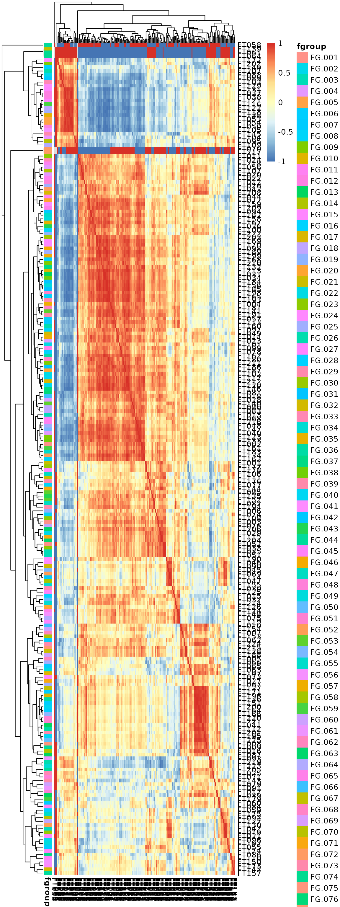
Correlation of features based on feature abundances.
Some large correlations can be observed for several groups of features, but many of them are not within the same feature group as defined in the previous section (i.e. are not eluting at the same time).
Below we use the groupFeatures with the AbundanceSimilarityParam to group features with a correlation higher than 0.7 including both detected and filled-in signal. Whether filled-in or only detected signal should be used in the correlation analysis should be evaluated from data set to data set. By specifying transform = log2 we tell the function to log2 transform the abundance prior to the correlation analysis.
xdata <- groupFeatures(xdata, AbundanceSimilarityParam(threshold = 0.7,
                                                       transform = log2),
                       filled = TRUE)
table(featureGroups(xdata))
##
## FG.001.001 FG.001.002 FG.002.001 FG.002.002 FG.002.003 FG.003.001 FG.003.002
## 2 1 1 1 1 2 1
## FG.004.001 FG.005.001 FG.006.001 FG.006.002 FG.007.001 FG.007.002 FG.007.003
## 3 2 3 1 2 1 1
## FG.007.004 FG.008.001 FG.008.002 FG.008.003 FG.008.004 FG.009.001 FG.009.002
## 1 3 1 1 1 3 1
## FG.010.001 FG.011.001 FG.011.002 FG.011.003 FG.012.001 FG.013.001 FG.013.002
## 2 2 2 1 3 2 1
## FG.013.003 FG.014.001 FG.014.002 FG.015.001 FG.015.002 FG.015.003 FG.015.004
## 1 2 1 2 1 1 1
## FG.016.001 FG.016.002 FG.017.001 FG.017.002 FG.018.001 FG.018.002 FG.018.003
## 2 1 2 1 2 1 1
## FG.018.004 FG.019.001 FG.019.002 FG.019.003 FG.020.001 FG.020.002 FG.021.001
## 1 1 1 1 2 1 1
## FG.021.002 FG.021.003 FG.022.001 FG.022.002 FG.022.003 FG.023.001 FG.023.002
## 1 1 1 1 1 2 1
## FG.024.001 FG.024.002 FG.024.003 FG.025.001 FG.025.002 FG.025.003 FG.025.004
## 1 1 1 2 1 1 1
## FG.025.005 FG.026.001 FG.026.002 FG.026.003 FG.027.001 FG.027.002 FG.027.003
## 1 1 1 1 1 1 1
## FG.028.001 FG.028.002 FG.029.001 FG.029.002 FG.030.001 FG.030.002 FG.031.001
## 2 1 2 2 1 1 3
## FG.032.001 FG.032.002 FG.032.003 FG.033.001 FG.033.002 FG.033.003 FG.033.004
## 1 1 1 1 1 1 1
## FG.034.001 FG.034.002 FG.034.003 FG.035.001 FG.035.002 FG.036.001 FG.036.002
## 1 1 1 1 1 2 1
## FG.037.001 FG.037.002 FG.038.001 FG.039.001 FG.040.001 FG.040.002 FG.041.001
## 2 1 2 2 2 2 1
## FG.041.002 FG.041.003 FG.042.001 FG.042.002 FG.043.001 FG.044.001 FG.044.002
## 1 1 1 1 2 2 1
## FG.044.003 FG.045.001 FG.045.002 FG.045.003 FG.045.004 FG.046.001 FG.047.001
## 1 1 1 1 1 2 1
## FG.047.002 FG.047.003 FG.048.001 FG.048.002 FG.048.003 FG.049.001 FG.049.002
## 1 1 1 1 1 2 1
## FG.050.001 FG.050.002 FG.051.001 FG.052.001 FG.052.002 FG.053.001 FG.053.002
## 1 1 2 2 1 2 1
## FG.053.003 FG.054.001 FG.054.002 FG.055.001 FG.055.002 FG.055.003 FG.056.001
## 1 1 1 1 1 1 1
## FG.056.002 FG.056.003 FG.057.001 FG.058.001 FG.058.002 FG.059.001 FG.059.002
## 1 1 2 1 1 1 1
## FG.059.003 FG.060.001 FG.060.002 FG.061.001 FG.061.002 FG.062.001 FG.062.002
## 1 2 1 2 1 1 1
## FG.063.001 FG.064.001 FG.064.002 FG.065.001 FG.065.002 FG.066.001 FG.066.002
## 2 1 1 2 1 1 1
## FG.067.001 FG.067.002 FG.068.001 FG.069.001 FG.070.001 FG.070.002 FG.071.001
## 1 1 3 2 1 1 2
## FG.071.002 FG.072.001 FG.072.002 FG.073.001 FG.073.002 FG.074.001 FG.075.001
## 1 2 1 1 1 2 1
## FG.076.001 FG.077.001
## 1 1Many of the larger retention time-based feature groups have been splitted into two or more sub-groups based on the correlation of their feature abundances. We evaluate this for one specific feature group "FG.040" by plotting their pairwise correlation.
fts <- grep("FG.040", featureGroups(xdata))
pairs(t(fvals[fts, ]), gap = 0.1, main = "FG.040")
Pairwise correlation plot for all features initially grouped into the feature group FG.040.
Indeed, correlations can be seen only between some of the features in this retention time feature group, e.g. between FT117 and FT120 and between FT195 and FT200. Note however that this abundance correlation suffers from relatively few samples (8 in total), and a relatively small variance in abundances across these samples.
After feature grouping by abundance correlation, the 225 features have been grouped into 170 feature groups.
Grouping of features by EIC correlation
The chromatographic peak shape of an ion of a compound should be highly similar to the elution pattern of this compound. Thus, features from the same compound are assumed to have similar peak shapes of their EICs within the same sample. Peak shape correlation can be performed with groupFeatures and the EicCorrelationParam. It is advisable to perform the peak shape correlation only on a subset of samples (because peak shape correlation is computationally intense and because chromatographic peaks of low intensity features are notoriously noisy). The EicCorrelationParam approach has thus the parameter n which allows to select the number of top samples (ordered by total intensity of feature abundances per feature group) on which the correlation should be performed. With an value of n = 3 for each feature group the 3 samples with the highest signal for all features in that group will be first identified and then within each of these samples a pairwise correlation will be performed between peak shapes of all features of the group. The resulting correlation coefficients from these 3 samples will then be reduced to a single correlation coefficient by taking the 75% quantile across the 3 samples. This value is then subsequently compared with the threshold correlation coefficient (parameter threshold) and only features are grouped together that have a correlation coefficient larger than this value.
Below we group the features based on their EIC correlation in the two samples with the highest total signal for the respective feature groups. We require the correlation of the peak shape to be higher than 0.7. With clean = TRUE we also ensure that only the signal within the actually detected chromatographic peaks is used.
xdata <- groupFeatures(xdata, EicCorrelationParam(threshold = 0.7, n = 2,
                                                  clean = TRUE))
##
|
| | 0%
|
|= | 1%
|
|== | 2%
|
|== | 3%
|
|== | 4%
|
|=== | 4%
|
|=== | 5%
|
|==== | 5%
|
|==== | 6%
|
|===== | 7%
|
|===== | 8%
|
|====== | 8%
|
|====== | 9%
|
|======= | 10%
|
|======= | 11%
|
|======== | 12%
|
|========= | 12%
|
|========= | 13%
|
|========== | 14%
|
|========== | 15%
|
|=========== | 15%
|
|=========== | 16%
|
|============ | 17%
|
|============ | 18%
|
|============= | 19%
|
|============== | 20%
|
|=============== | 21%
|
|=============== | 22%
|
|================ | 22%
|
|================ | 23%
|
|================ | 24%
|
|================= | 24%
|
|================= | 25%
|
|================== | 26%
|
|=================== | 27%
|
|=================== | 28%
|
|==================== | 28%
|
|===================== | 29%
|
|===================== | 30%
|
|====================== | 31%
|
|====================== | 32%
|
|======================= | 32%
|
|======================= | 33%
|
|======================== | 34%
|
|========================= | 35%
|
|========================= | 36%
|
|========================== | 36%
|
|========================== | 37%
|
|========================== | 38%
|
|=========================== | 38%
|
|=========================== | 39%
|
|============================ | 40%
|
|============================= | 41%
|
|============================= | 42%
|
|============================== | 42%
|
|============================== | 43%
|
|============================== | 44%
|
|=============================== | 44%
|
|=============================== | 45%
|
|================================ | 45%
|
|================================ | 46%
|
|================================= | 47%
|
|================================= | 48%
|
|================================== | 48%
|
|=================================== | 50%
|
|=================================== | 51%
|
|==================================== | 52%
|
|===================================== | 52%
|
|===================================== | 53%
|
|====================================== | 54%
|
|======================================= | 55%
|
|======================================= | 56%
|
|======================================== | 56%
|
|======================================== | 57%
|
|======================================== | 58%
|
|========================================= | 58%
|
|========================================= | 59%
|
|========================================== | 60%
|
|=========================================== | 61%
|
|=========================================== | 62%
|
|============================================ | 62%
|
|============================================ | 64%
|
|============================================= | 64%
|
|============================================= | 65%
|
|============================================== | 65%
|
|============================================== | 66%
|
|=============================================== | 67%
|
|=============================================== | 68%
|
|================================================ | 68%
|
|================================================ | 69%
|
|================================================= | 69%
|
|================================================= | 70%
|
|================================================= | 71%
|
|================================================== | 71%
|
|================================================== | 72%
|
|=================================================== | 72%
|
|=================================================== | 73%
|
|==================================================== | 74%
|
|===================================================== | 75%
|
|===================================================== | 76%
|
|====================================================== | 76%
|
|====================================================== | 77%
|
|====================================================== | 78%
|
|======================================================= | 78%
|
|======================================================= | 79%
|
|======================================================== | 80%
|
|========================================================= | 81%
|
|========================================================= | 82%
|
|========================================================== | 82%
|
|========================================================== | 83%
|
|========================================================== | 84%
|
|=========================================================== | 84%
|
|============================================================ | 86%
|
|============================================================= | 87%
|
|============================================================== | 88%
|
|=============================================================== | 89%
|
|=============================================================== | 90%
|
|=============================================================== | 91%
|
|================================================================ | 92%
|
|================================================================= | 92%
|
|================================================================= | 93%
|
|================================================================== | 94%
|
|================================================================== | 95%
|
|=================================================================== | 95%
|
|=================================================================== | 96%
|
|==================================================================== | 96%
|
|==================================================================== | 97%
|
|==================================================================== | 98%
|
|===================================================================== | 99%
|
|======================================================================| 100%This is the most computationally intense approach since it involves also loading the raw MS data to extract the ion chromatograms for each feature. The results of the grouping are shown below.
table(featureGroups(xdata))##
## FG.001.001.001 FG.001.002.001 FG.002.001.001 FG.002.002.001 FG.002.003.001
## 2 1 1 1 1
## FG.003.001.001 FG.003.002.001 FG.004.001.001 FG.005.001.001 FG.006.001.001
## 2 1 3 2 3
## FG.006.002.001 FG.007.001.001 FG.007.002.001 FG.007.003.001 FG.007.004.001
## 1 2 1 1 1
## FG.008.001.001 FG.008.001.002 FG.008.002.001 FG.008.003.001 FG.008.004.001
## 2 1 1 1 1
## FG.009.001.001 FG.009.002.001 FG.010.001.001 FG.010.001.002 FG.011.001.001
## 3 1 1 1 2
## FG.011.002.001 FG.011.003.001 FG.012.001.001 FG.013.001.001 FG.013.002.001
## 2 1 3 2 1
## FG.013.003.001 FG.014.001.001 FG.014.002.001 FG.015.001.001 FG.015.002.001
## 1 2 1 2 1
## FG.015.003.001 FG.015.004.001 FG.016.001.001 FG.016.002.001 FG.017.001.001
## 1 1 2 1 2
## FG.017.002.001 FG.018.001.001 FG.018.002.001 FG.018.003.001 FG.018.004.001
## 1 2 1 1 1
## FG.019.001.001 FG.019.002.001 FG.019.003.001 FG.020.001.001 FG.020.001.002
## 1 1 1 1 1
## FG.020.002.001 FG.021.001.001 FG.021.002.001 FG.021.003.001 FG.022.001.001
## 1 1 1 1 1
## FG.022.002.001 FG.022.003.001 FG.023.001.001 FG.023.002.001 FG.024.001.001
## 1 1 2 1 1
## FG.024.002.001 FG.024.003.001 FG.025.001.001 FG.025.001.002 FG.025.002.001
## 1 1 1 1 1
## FG.025.003.001 FG.025.004.001 FG.025.005.001 FG.026.001.001 FG.026.002.001
## 1 1 1 1 1
## FG.026.003.001 FG.027.001.001 FG.027.002.001 FG.027.003.001 FG.028.001.001
## 1 1 1 1 2
## FG.028.002.001 FG.029.001.001 FG.029.002.001 FG.029.002.002 FG.030.001.001
## 1 2 1 1 1
## FG.030.002.001 FG.031.001.001 FG.032.001.001 FG.032.002.001 FG.032.003.001
## 1 3 1 1 1
## FG.033.001.001 FG.033.002.001 FG.033.003.001 FG.033.004.001 FG.034.001.001
## 1 1 1 1 1
## FG.034.002.001 FG.034.003.001 FG.035.001.001 FG.035.002.001 FG.036.001.001
## 1 1 1 1 1
## FG.036.001.002 FG.036.002.001 FG.037.001.001 FG.037.002.001 FG.038.001.001
## 1 1 2 1 2
## FG.039.001.001 FG.039.001.002 FG.040.001.001 FG.040.002.001 FG.041.001.001
## 1 1 2 2 1
## FG.041.002.001 FG.041.003.001 FG.042.001.001 FG.042.002.001 FG.043.001.001
## 1 1 1 1 2
## FG.044.001.001 FG.044.001.002 FG.044.002.001 FG.044.003.001 FG.045.001.001
## 1 1 1 1 1
## FG.045.002.001 FG.045.003.001 FG.045.004.001 FG.046.001.001 FG.047.001.001
## 1 1 1 2 1
## FG.047.002.001 FG.047.003.001 FG.048.001.001 FG.048.002.001 FG.048.003.001
## 1 1 1 1 1
## FG.049.001.001 FG.049.002.001 FG.050.001.001 FG.050.002.001 FG.051.001.001
## 2 1 1 1 2
## FG.052.001.001 FG.052.002.001 FG.053.001.001 FG.053.001.002 FG.053.002.001
## 2 1 1 1 1
## FG.053.003.001 FG.054.001.001 FG.054.002.001 FG.055.001.001 FG.055.002.001
## 1 1 1 1 1
## FG.055.003.001 FG.056.001.001 FG.056.002.001 FG.056.003.001 FG.057.001.001
## 1 1 1 1 2
## FG.058.001.001 FG.058.002.001 FG.059.001.001 FG.059.002.001 FG.059.003.001
## 1 1 1 1 1
## FG.060.001.001 FG.060.001.002 FG.060.002.001 FG.061.001.001 FG.061.002.001
## 1 1 1 2 1
## FG.062.001.001 FG.062.002.001 FG.063.001.001 FG.064.001.001 FG.064.002.001
## 1 1 2 1 1
## FG.065.001.001 FG.065.002.001 FG.066.001.001 FG.066.002.001 FG.067.001.001
## 2 1 1 1 1
## FG.067.002.001 FG.068.001.001 FG.068.001.002 FG.069.001.001 FG.070.001.001
## 1 2 1 2 1
## FG.070.002.001 FG.071.001.001 FG.071.001.002 FG.071.002.001 FG.072.001.001
## 1 1 1 1 1
## FG.072.001.002 FG.072.002.001 FG.073.001.001 FG.073.002.001 FG.074.001.001
## 1 1 1 1 2
## FG.075.001.001 FG.076.001.001 FG.077.001.001
## 1 1 1In most cases, pre-defined feature groups (by the abundance correlation) were not further subdivided. Below we evaluate some of the feature groups starting with FG.007.02 which was split into two different feature groups based on EIC correlation. We first extract the EICs for all features from this initial feature group. With n = 1 we specify to extract the EIC only from the sample with the highest intensity.
fts <- grep("FG.008.001", featureGroups(xdata))
eics <- featureChromatograms(xdata, features = fts,
                             filled = TRUE, n = 1)
Next we plot the EICs using a different color for each of the subgroups.
cols <- c("#ff000080", "#00ff0080")
names(cols) <- unique(featureGroups(xdata)[fts])

par(mfrow = c(1, 2))
plotOverlay(eics, col = cols[featureGroups(xdata)[fts]], lwd = 2)
plotOverlay(normalize(eics), col = cols[featureGroups(xdata)[fts]], lwd = 2)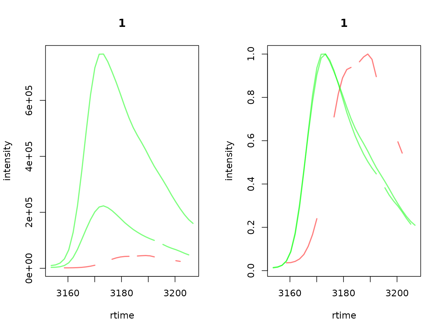
EICs of features from feature group FG.008.001, colors label different feature sub-groups. Shown are the actual intensities (left) and intensities normalized to 1 (right).
One feature initially grouped together with all other features based on the abundance correlation was separated from them based on the EIC correlation. In addition, two features seem to have only a single peak, while the others have a double peak. Here it is not clear if it would be better to include the feature labeled in green in the main feature group, or if the feature group should be further splitted based on the presence of the additional peak. Since these EICs were all extracted from the same sample, the shift observed for the green colored feature the can not be the result from a mis-alignment hence suggesting that this feature might be indeed be from a different compound.
We evaluate next the sub-grouping in another feature group.
fts <- grep("FG.068.001", featureGroups(xdata))
eics <- featureChromatograms(xdata, features = fts,
                             filled = TRUE, n = 1)
Next we plot the EICs using a different color for each of the subgroups.
cols <- c("#ff000080", "#00ff0080")
names(cols) <- unique(featureGroups(xdata)[fts])

par(mfrow = c(1, 2))
plotOverlay(eics, col = cols[featureGroups(xdata)[fts]], lwd = 2)
plotOverlay(normalize(eics), col = cols[featureGroups(xdata)[fts]], lwd = 2)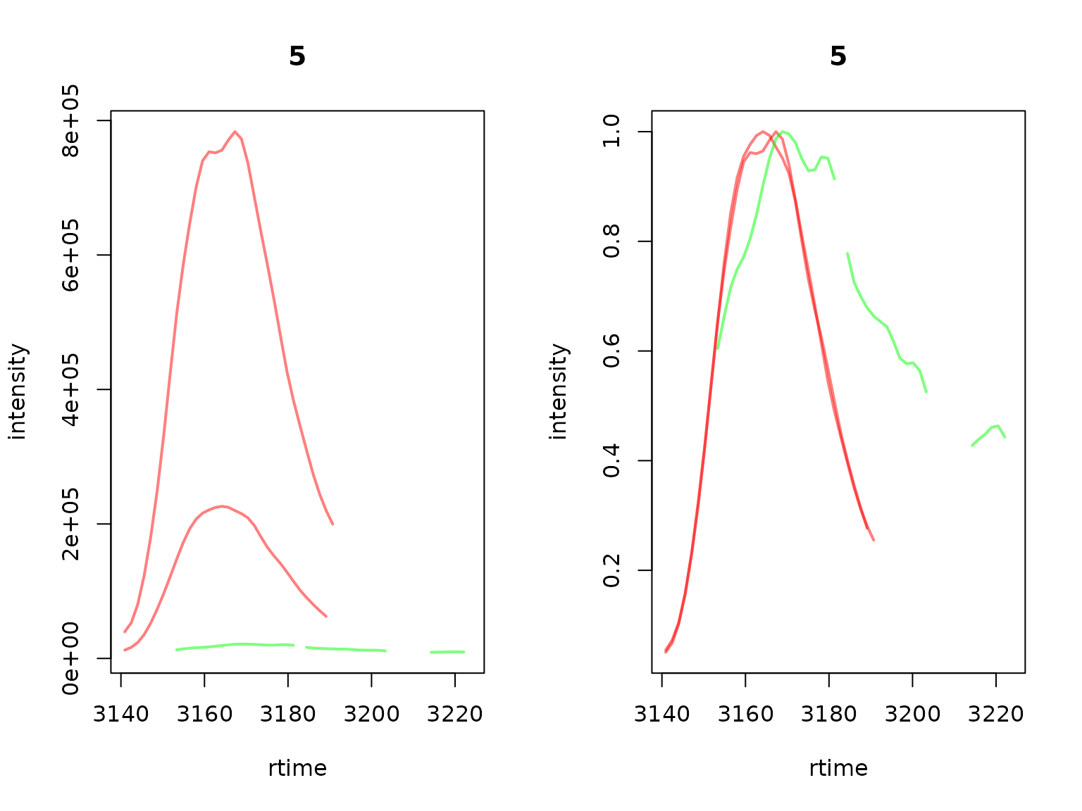
EICs of features from feature group FG.068.001, colors label different feature sub-groups. Shown are the actual intensities (left) and intensities normalized to 1 (right).
Based on the EIC correlation, the initial feature group FG.068.001 was grouped into two separate sub-groups.
The grouping based on EIC correlation on the pre-defined feature groups from the previous sections grouped the 225 features into 183 feature groups.
Grouping of subsets of features
In the previous sections we were always considering all features from the data set, but sometimes it could be desirable to just group a pre-defined set of features, for example features found to be of particular interest in a certain experiment (e.g. significant features). This can be easily achieved by assigning the features of interest to a initial feature group, using NA as group ID for all other features.
To illustrate this we reset all feature groups by setting them to NA and assign our features of interest (in this example just 30 randomly selected features) to an initial feature group "FG".
featureDefinitions(xdata)$feature_group <- NA_character_

set.seed(123)
fts_idx <- sample(1:nrow(featureDefinitions(xdata)), 30)
featureDefinitions(xdata)$feature_group[fts_idx] <- "FG"
Any call to groupFeatures would now simply sub-group this set of 30 features. Any feature which has an NA in the "feature_group" column will be ignored.
xdata <- groupFeatures(xdata, SimilarRtimeParam(diffRt = 20))
xdata <- groupFeatures(xdata, AbundanceSimilarityParam(threshold = 0.7))
table(featureGroups(xdata))
##
## FG.001.001 FG.001.002 FG.002.001 FG.003.001 FG.003.002 FG.004.001 FG.004.002
## 2 2 4 2 1 1 1
## FG.004.003 FG.005.001 FG.005.002 FG.006.001 FG.006.002 FG.007.001 FG.008.001
## 1 1 1 1 1 2 1
## FG.009.001 FG.010.001 FG.011.001 FG.012.001 FG.013.001 FG.014.001 FG.015.001
## 1 1 1 1 1 1 1
## FG.016.001 FG.017.001
## 1 1Session information
## R Under development (unstable) (2021-02-25 r80035)
## Platform: x86_64-pc-linux-gnu (64-bit)
## Running under: Ubuntu 20.04.2 LTS
##
## Matrix products: default
## BLAS/LAPACK: /usr/lib/x86_64-linux-gnu/openblas-pthread/libopenblasp-r0.3.8.so
##
## locale:
##  [1] LC_CTYPE=en_US.UTF-8       LC_NUMERIC=C
##  [3] LC_TIME=en_US.UTF-8        LC_COLLATE=en_US.UTF-8
##  [5] LC_MONETARY=en_US.UTF-8    LC_MESSAGES=C
##  [7] LC_PAPER=en_US.UTF-8       LC_NAME=C
##  [9] LC_ADDRESS=C               LC_TELEPHONE=C
## [11] LC_MEASUREMENT=en_US.UTF-8 LC_IDENTIFICATION=C
##
## attached base packages:
## [1] stats4    parallel  stats     graphics  grDevices utils     datasets
## [8] methods   base
##
## other attached packages:
##  [1] pheatmap_1.0.12       CompMetaboTools_0.3.2 MsFeatures_0.99.1
##  [4] faahKO_1.31.0         xcms_3.13.5           MSnbase_2.17.8
##  [7] ProtGenerics_1.23.7   S4Vectors_0.29.7      mzR_2.25.3
## [10] Rcpp_1.0.6            Biobase_2.51.0        BiocGenerics_0.37.1
## [13] BiocParallel_1.25.4   BiocStyle_2.19.1
##
## loaded via a namespace (and not attached):
##  [1] bitops_1.0-6                matrixStats_0.58.0
##  [3] fs_1.5.0                    doParallel_1.0.16
##  [5] RColorBrewer_1.1-2          rprojroot_2.0.2
##  [7] GenomeInfoDb_1.27.6         tools_4.1.0
##  [9] utf8_1.1.4                  R6_2.5.0
## [11] affyio_1.61.0               colorspace_2.0-0
## [13] compiler_4.1.0              MassSpecWavelet_1.57.0
## [15] preprocessCore_1.53.2       textshaping_0.3.1
## [17] desc_1.2.0                  DelayedArray_0.17.9
## [19] bookdown_0.21               scales_1.1.1
## [21] DEoptimR_1.0-8              robustbase_0.93-7
## [23] affy_1.69.0                 pkgdown_1.6.1.9000
## [25] systemfonts_1.0.1           stringr_1.4.0
## [27] digest_0.6.27               rmarkdown_2.7
## [29] XVector_0.31.1              pkgconfig_2.0.3
## [31] htmltools_0.5.1.1           MatrixGenerics_1.3.1
## [33] highr_0.8                   fastmap_1.1.0
## [35] limma_3.47.8                rlang_0.4.10
## [37] impute_1.65.0               farver_2.1.0
## [39] mzID_1.29.0                 RCurl_1.98-1.2
## [41] magrittr_2.0.1              GenomeInfoDbData_1.2.4
## [43] MALDIquant_1.19.3           Matrix_1.3-2
## [45] munsell_0.5.0               fansi_0.4.2
## [47] MsCoreUtils_1.3.3           lifecycle_1.0.0
## [49] vsn_3.59.1                  stringi_1.5.3
## [51] yaml_2.2.1                  MASS_7.3-53.1
## [53] SummarizedExperiment_1.21.1 zlibbioc_1.37.0
## [55] plyr_1.8.6                  grid_4.1.0
## [57] crayon_1.4.1                lattice_0.20-41
## [59] knitr_1.31                  pillar_1.5.0
## [61] GenomicRanges_1.43.3        codetools_0.2-18
## [63] XML_3.99-0.5                glue_1.4.2
## [65] evaluate_0.14               pcaMethods_1.83.0
## [67] BiocManager_1.30.10         vctrs_0.3.6
## [69] foreach_1.5.1               gtable_0.3.0
## [71] RANN_2.6.1                  clue_0.3-58
## [73] assertthat_0.2.1            cachem_1.0.4
## [75] ggplot2_3.3.3               xfun_0.21
## [77] ragg_1.1.1                  ncdf4_1.17
## [79] tibble_3.1.0                iterators_1.0.13
## [81] memoise_2.0.0               IRanges_2.25.6
## [83] cluster_2.1.1               ellipsis_0.3.1