Pedigree analysis and familial aggregation methods
FAData-analysis.RdVarious functions to perform pedigree analyses and to investigate familial clustering of e.g. cancer cases.
binomialTest(object, trait, traitName, global = FALSE, prob = NULL,
    alternative = c("greater", "less", "two.sided"))

estimateTimeAtRisk(startDate=NULL, startDateFormat="%Y-%m-%d",
                   endDate=NULL, endDateFormat="%Y-%m-%d",
                   incidenceDate=NULL, incidenceDateFormat="%Y-%m-%d",
                   deathDate=NULL, deathDateFormat="%Y-%m-%d",
                   allowNegative=FALSE, affected=NULL,
                   incidenceSubtract=0.5)

factor2matrix(x)

# S4 method for FAData
familialIncidenceRate(object, trait=NULL,
                                         timeAtRisk=NULL)

# S4 method for FAData
familialIncidenceRateTest(object, trait=NULL,
                                            nsim=50000, traitName=NULL,
                                            timeAtRisk=NULL,
                                            strata=NULL, ...)

# S4 method for FAData
fsir(object, trait=NULL, lambda=NULL, timeInStrata=NULL)

# S4 method for FAData
fsirTest(object, trait=NULL, nsim=50000, traitName=NULL,
                            lambda=NULL, timeInStrata=NULL,
                            strata=NULL, ...)

# S4 method for FAData
genealogicalIndexTest(object, trait, nsim=50000,
                                         traitName, perFamilyTest=FALSE,
                                         controlSetMethod="getAll",
                                         rm.singletons=TRUE, strata=NULL, ...)

# S4 method for FAData
kinshipGroupTest(object, trait, nsim=50000,
                                    traitName, strata=NULL, ...)

# S4 method for FAData
kinshipSumTest(object, trait, nsim=50000,
                                  traitName, strata=NULL, ...)

# S4 method for FAData
probabilityTest(object, trait, cliques,
                                   nsim=50000, traitName,
                                   ...)

sliceAge(x, slices=c(0, 40, Inf))
<!-- %connectedSubgraph(graph, nodes, mode="all", all.nodes=TRUE, ifnotfound) -->
Arguments
| affected | For |
|---|---|
| allowNegative | For |
| alternative | For |
| cliques | A named numeric or characted vector or factor with the names corresponding to ids of the individuals in the pedigree. The ids will be internally matched and sub-set to the ids available in the pedigree. |
| controlSetMethod | For |
| deathDate | For |
| deathDateFormat | For |
| endDate | For |
| endDateFormat | For |
| global | For |
| incidenceDate | For |
| incidenceDateFormat | For |
| incidenceSubtract | For |
| lambda | Numeric vector with the incidence rates per stratum from the
population. The length of this vector has to match the number of
columns of argument |
| nsim | The number of simulations. |
| object | The |
| perFamilyTest | For |
| prob | For |
| rm.singletons | For |
| slices | For |
| startDate | For |
| startDateFormat | For |
| strata | For |
| timeAtRisk | A numeric vector specifying the time at risk for each
individual. The definition for this variable is taken from Kerber
(1995). See description of the method below for more information.
|
| timeInStrata | For |
| trait | A named numeric vector (values If trait is not specified, the trait information stored within the
|
| traitName | The name of the trait (optional). |
| x | For |
| ... | For For |
Details
Stratified sampling: some of the familial aggregation methods allow to use stratified sampling for the Monte Carlo simulations. In stratified sampling, the same number of random samples will be selected within each class/stratum then there are among the affected. As example, if 5 female and 2 male individuals are affected in the analysed trait and sex stratified sampling is performed, in each permuatation the same number of random samples in each group (i.e. 5 females and 2 males) are selected.
A note on singletons: for all per-individual measures, unconnected individuals within the pedigree are automatically excluded from the calculations as no kinship based statistic can be estimated for them since they do, by definition, not share kinship with any other individual in the pedigree.
Familial aggregation methods
- binomialTest
Evaluate whether the number of affected in a trait are higher than expected by chance using a simple binomial test. In contrast to most other methods presented here, this does not use the kinship between affected individuals, but simply performs a binomial test for each family considering the numbers of affected within the family, the size of the family and the global probability of being affected. The latter is by default calculated on the data set (ratio between the total number of affected in the pedigree and the total number of phenotyped individuals), can however also be specified with the
probargument. The test is performed using thebinom.test. The function returns aFABinTestResultsobject.- familialIncidenceRate
Calculate the familial incidence rate (FIR, or FR) as defined in [Kerber 1995], formula (3). The FIR is an estimate for the risk per gene-time for each individual for a certain disease (trait) given the disease experience in the cohort. The measure considers the kinship of each individual with any affected individual in the pedigree and the time at risk for each individual. Internally, the function first excludes individuals from the test which have a missing value (
NA) either in the argumenttraitor in the argumenttimeAtRisk. Next, the thus reduced pedigree, is further cleaned by removing all resulting singletons (i.e. individuals that do not share kinship with any other individual in the above reduced data set). The method returns a vector with the FIR value for each individual. Individuals that were excluded from the test as described above habe an FIR ofNA.- familialIncidenceRateTest
Calculates the familial incidence rate for each individual and in addition assesses the significance of these based on Monte Carlo simulations. See
FAIncidenceRateResultsfor more details. The method returns aFAIncidenceRateResultsobject.- fsir
Calculate the familial standardized incidence rate (FSIR) as defined in [Kerber, 1995], formula (4). The FSIR weights the disease status of relatives based on their degree of relatedness with the proband [Kerber, 1995]. Formally, the FSIR is defined as the standardized incidence ratio (SIR) or standardized morality ratio in epidemiology, i.e. as the ratio between the observed and expected number of cases, only that both are in addition also weighted by the degree of relatedness (i.e. kinship value) between individuals in the pedigree. Similar to
familialIncidenceRate, the function excludes individuals with missing values in any of the argumentstrait,timeInStrata(and optionallystrata) and all individuals that do not share any kinship with any other individual in the pedigree after removing the above individuals. The method returns a vector with the FSIR value for each individual. Individuals excluded as above describe have a FSIR value ofNA.- fsirTest
Calculates the familial standardized incidence rate (FSIR) for each individual and in addition assesses the significance of these based on Monte Carlo simulations. See
FAStdIncidenceRateResultsfor more details. The method returns aFAStdIncidenceRateResultsobject.- genealogicalIndexTest
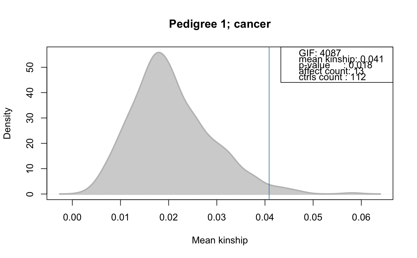
Performs the genealogical index analysis from [Hill 1980] (also known as the genealogical index of familiality or
genetic index of familiality) to identify familial clustering of traits (e.g. cancers etc). This test calculates the mean kinship among affected individuals in a pedigree along with mean kinships of equal sized random control sets drawn form the pedigree. The distribution of average kinship values among these random sets is used to estimate the probability that the observed mean kinship between the affected individuals is due to chance. ThecontrolSetMethodargument allows to specify the method to define sets of matched control individuals in a pedigree or family. Note that by default singletons (i.e. unconnected individuals in the pedigree) are removed from the pedigree prior the analysis. Setrm.singletons=FALSEif you do not want them to be removed. The method can also be performed separately for each family within the larger pedigree (perFamilyTest=TRUEto evaluate the presence of clustered affected within each family). In this case it is also possible to usecontrolSetMethod="getGenerationMatched"orcontrolSetMethod="getGenerationSexMatched", which allows to draw random control samples from the same generation(s) than the affected are. Stratified random sampling can be performed with thestrataargument. See details for more information. The function returns aFAGenIndexResultsobject.- kinshipGroupTest
Performs a familial aggregation test on a subset of a family. The idea behind this test is to narrow down the set of controls for each affected individual by considering only individuals that are as closely related as the most distant affected individual. This strategy incorporates more the family structure of the cases and is meant to be an alternative to the
kinshipSumTestmethod. Initially, for an affected individual i a group C(i) is created that contains all individuals that share kinship as far as the most distantly related affected individual. This cluster can be interpreted as a circle that is centered at individual i with radius equal to the most distantly related case. Therefore, the cluster defines a narrowed, individual-specific set of individuals in which the phenotype is assumed to have been passed on. Groups consisting of the same set of affected individuals are reduced to a single group (i.e. the group with the smallest total number of individuals). Based on this definition of groups C(i), we compute two statistics by performing Monte Carlo simulations (which optionally allow to perform stratified random sampling). During each simulation step affected cases are randomly sampled from the population. 1. The ratio test counts per group C(i) the number of times we observe a higher number of affected individuals in the simulation than in the observed case. Dividing this number by the number of simulation steps yields immediately the p-value that describes the event to observe by chance a higher number of affected individuals than in the given case. 2. The kinship test addresses the degree of relatedness within the simulated set by a counting method where we count the number of times in a simulation step there is a pair of affected individuals that are more closely related than in the observed group C(i). In case the closest degree of relatedness is equal in both the simulation step and the observed case, we look at the number of pairs found in both and count it if this number is higher in the simulation step. Again, dividing this count by the number of simulation steps readily yields a p-value. See also the methodrunSimulationforFAKinGroupResults. The function returns aFAKinGroupResultsobject.- kinshipSumTest
Performs a test for familial aggregation based on the sum of kinship values between affected cases. This test highlights individuals that exhibit a higher than chance relationship to other affected individuals, therefore highlighting individuals within families aggregating the phenotype. To achieve this, for each affected individual the sum of kinship values to all other affected cases is computed. In a Monte Carlo simulation this is repeated with the same number of cases (and optionally stratified with the
strataargument), and the resulting background distribution is used to compute p-values for the kinship sums obtained from the observed cases. See also the methodrunSimulationforFAKinSumResults. The function returns aFAKinSumResultsobject.- probabilityTest
DEPRECATED: this test will be removed in Bioconductor version 3.8 due to problems and incompatibilities of the
gappackage on MS Windows systems. This is only a convience method that calls thegappackage's methodpfc.simto compute probabilities of familial clustering of phenotypes [Yu and Zelterman (2002)]. One drawback of that method is that it is limited to families with at most 22 individuals. Thus, pedigrees need to be split with specialized software such as Jenti [Falchi and Fuchsberger ea. (2008)], which within large families define cliques that can then be used as input to this algorithm. See also methodrunSimulationforFAProbResults. The function returns aFAProbResultsobject.
Utility functions
- factor2matrix
Converts a factor into a matrix with columns corresponding to the levels and values (cell row i, column j) being either 0 or 1 depending on whether the ith factor was of the level j. See examples below for in or
FAStdIncidenceRateResults.- estimateTimeAtRisk
Function to calculate the time at risk based on the start date of the study or the birth date of an individual (
startDate) and the study's end date (endDate), the date of an incidence (e.g. date of diagnosis of a cancerincidenceDate) or the death of the individual (deathDate). The time at risk for each individual is calculated as the minimal time period betweenstartDateand any ofendDate,incidenceDateordeathDate. Thus it is also possible to provide just theendDatealong with thestartDate, in which case theendDateshould be the earliest time point of: end date of the study, incidence date or date of death. For affected individuals (those for which either an incidence date is provided or the value in the optional argumentaffectedisTRUEor bigger than 0), by default half of the time unit is subtracted. For example, a individual that has an incidence after 2 days is 1.5 days at risk. The proportion of the time unit to subtract can be specified with the argumentincidenceSubtract. The function returns a numeric vector with the time at risk in days.- sliceAge
Generates a matrix with columns corresponding to age slices/strata defined by argument
slicesand rows to individuals. Each cell in a row represents the time spent by the individual in the age slice/strata. See example below.
Value
Refer to the method and function description above for detailed information on the returned result object.
References
Rainer J, Talliun D, D'Elia Y, Domingues FS and Weichenberger CX (2016) FamAgg: an R package to evaluate familial aggregation of traits in large pedigrees. Bioinformatics.
Hill, J.R. (1980) A survey of cancer sites by kinship in the Utah Mormon population. In Cairns J, Lyon JL, Skolnick M (eds): Cancer Incidence in Defined Populations. Banbury Report 4. Cold Spring Harbor, NY: Cold Spring Harbor Laboratory Press, pp 299--318.
Kerber, R.A. (1995) Method for calculating risk associated with family history of a disease. Genet Epidemiol, pp 291--301.
Yu, C. and Zelterman, D. (2002) Statistical inference for familial disease clusters. Biometrics, pp 481--491
Falchi, M. and Fuchsberger, C. (2008) Jenti: an efficient tool for mining complex inbred genealogies. Bioinformatics, pp 724--726
See also
Examples
########################## ## ## Defining a small pedigree ## ## load the Minnesota Breast Cancer record and subset to the ## first families. data(minnbreast) mbsub <- minnbreast[minnbreast$famid==4 | minnbreast$famid==5 | minnbreast$famid==14 | minnbreast$famid==8, ] mbped <- mbsub[, c("famid", "id", "fatherid", "motherid", "sex")] ## renaming column names colnames(mbped) <- c("family", "id", "father", "mother", "sex") ## create the FAData object fad <- FAData(pedigree=mbped)#>#>## We specify the cancer trait. tcancer <- mbsub$cancer names(tcancer) <- mbsub$id ########################## ## ## Familial Incidence Rate ## ## Calculate the FR for each individual given the affected status of ## each individual in trait cancer and the time at risk for each ## participant. We use column "endage" in the minnbreast data.frame ## that specifies the age at the last follow-up or incident cancer as a ##rather impresice estimate for time at risk. fr <- familialIncidenceRate(fad, trait=tcancer, timeAtRisk=mbsub$endage)#>#>#>#>#>#>#>#>## Perform in addition Monte Carlo simulations to assess the significance ## for the familial incidence rates. frRes <- familialIncidenceRateTest(fad, trait=tcancer, timeAtRisk=mbsub$endage, nsim=500)#>#>#>#>#>#>#>#>#> trait_name total_phenotyped total_affected total_tested id family #> 446 NA 129 15 88 446 14 #> 449 NA 129 15 88 449 14 #> 453 NA 129 15 88 453 14 #> 445 NA 129 15 88 445 14 #> 454 NA 129 15 88 454 14 #> 447 NA 129 15 88 447 14 #> fir pvalue padj #> 446 0.007424662 0.002 0.1173333 #> 449 0.006915362 0.004 0.1173333 #> 453 0.006629813 0.004 0.1173333 #> 445 0.006758000 0.008 0.1760000 #> 454 0.006481794 0.014 0.2464000 #> 447 0.005487605 0.028 0.4000000########################## ## ## Familial Standardized Incidence Rate: ## Please see examples of FAStdIncidenceRateResults. ########################## ## ## Perform familial aggregation analyses using the genealogical index ## gi <- genealogicalIndexTest(fad, trait=tcancer, traitName="cancer", nsim=500)#>#>#>#>#>#>result(gi)#> trait_name total_phenotyped total_affected entity_id entity_ctrls #> 1 cancer 129 15 1 112 #> entity_affected genealogical_index pvalue padj #> 1 13 4086.538 0.018 0.018## A significant clustering of cancer cases was identified in the ## analyzed pedigree. ## Plotting the observed mean kinship and the distribution of mean kinship ## from the random sampling. plotRes(gi)########################## ## ## Perform familial aggregation analysis using the kinship sum test ## kcr <- kinshipSumTest(fad, trait=tcancer, traitName="cancer", nsim=500)#>#>#>#>kcr#> FAKinSumResults object with: #> * Pedigree of length 191. #> * Number of unique individuals: 191. #> * Number of families: 4. #> * Number of individuals in largest family: 70. #> * Number of individuals in smallest family: 38. #> Information on trait 'cancer' #> * Number of non-NA values: 129. #> * Number of non-zero values: 15. #> Result info: #> * Number of rows of the result data.frame: 15. #> * Number of simulations: 500.#> trait_name total_phenotyped total_affected affected_id family affected #> 447 cancer 129 15 447 14 15 #> 450 cancer 129 15 450 14 15 #> 451 cancer 129 15 451 14 15 #> 452 cancer 129 15 452 14 15 #> 142 cancer 129 15 142 8 15 #> 444 cancer 129 15 444 14 15 #> kinship_sum freq pvalue padj #> 447 1.000 0.2133333 0.004266667 0.0565 #> 450 0.875 0.6800000 0.015066667 0.0565 #> 451 0.875 0.6800000 0.015066667 0.0565 #> 452 0.875 0.6800000 0.015066667 0.0565 #> 142 0.625 2.9600000 0.078000000 0.1950 #> 444 0.625 2.9600000 0.078000000 0.1950########################## ## ## Perform familial aggregation analysis using the kinship group test, ## stratifying by sex ## kr <- kinshipGroupTest(fad, trait=tcancer, traitName="cancer", nsim=500, strata=fad$sex)#>#>#>#>#>#>#>#>kr#> FAKinGroupResults object with: #> * Pedigree of length 191. #> * Number of unique individuals: 191. #> * Number of families: 4. #> * Number of individuals in largest family: 70. #> * Number of individuals in smallest family: 38. #> Information on trait 'cancer' #> * Number of non-NA values: 129. #> * Number of non-zero values: 15. #> Result info: #> * Dimension of result data.frame: 3. #> * Dimension of result data.frame: 14. #> * Number of simulations: 500.#> trait_name total_phenotyped total_affected phenotyped affected group_id #> 447 cancer 129 15 43 11 447 #> 136 cancer 129 15 43 11 136 #> 11 cancer 129 15 43 11 11 #> family group_phenotyped group_affected ratio_pvalue ratio_padj mean_kinship #> 447 14 12 5 0.006 0.018 0.2500000 #> 136 8 19 4 0.178 0.267 0.1666667 #> 11 4 12 2 0.550 0.550 0.1250000 #> kinship_pvalue kinship_padj #> 447 0.000 0.000 #> 136 0.154 0.231 #> 11 0.490 0.490########################## ## ## Estimate the time at risk given ## ## Define some birth dates and incidence dates and end date of study bdates <- c("2012-04-17", "2014-05-29", "1999-12-31", "2002-10-10") idates <- c(NA, NA, "2007-07-13", "2013-12-23") edates <- rep("2015-09-15", 4) ## Estimate the time at risk. The time period is returned in days. riskDays <- estimateTimeAtRisk(startDate=bdates, incidenceDate=idates, endDate=edates)#>#>#>#>#>#>riskDays#> [1] 1246.0 474.0 2750.5 4091.5########################## ## ## Define the time spent in an age stratum given the indivduals' ## age at incidence or end of study. head(mbsub$endage)#> [1] NA 78.05886 55.50000 48.00000 75.00342 53.63997## We "slice" the age in specified intervals/slices stratAge <- sliceAge(mbsub$endage, slices=c(0, 40, 60, Inf)) head(stratAge)#> (0, 40] (40, 60] (60, Inf] #> [1,] NA NA NA #> [2,] 40 20.00000 18.05886 #> [3,] 40 15.50000 0.00000 #> [4,] 40 8.00000 0.00000 #> [5,] 40 20.00000 15.00342 #> [6,] 40 13.63997 0.00000## The first column lists the number of years spent in the first age ## stratum (0 < age <= 40) and the second in the second stratum ## (40 < age <= Inf) ## We could also stratify the disk days from above in per year strata. sliceAge(riskDays/365, slices=c(0, 2.5, 5, 10, 20))#> (0, 2.5] (2.5, 5] (5, 10] (10, 20] #> [1,] 2.50000 0.9136986 0.000000 0.000000 #> [2,] 1.29863 0.0000000 0.000000 0.000000 #> [3,] 2.50000 2.5000000 2.535616 0.000000 #> [4,] 2.50000 2.5000000 5.000000 1.209589########################## ## ## Simple example for factor2matrix: generate a matrix for factor $sex head(factor2matrix(fad$sex))#> M F #> 1 1 0 #> 2 0 1 #> 3 0 1 #> 4 0 1 #> 5 1 0 #> 6 1 0